Journal
This is my lab Journal, Here I’ve wrote some R scripts that I used for the analysis of my data during my research, I hope You will find this Usefull. The problems and tasks may not be in a chronological order so feel free to surf the whole page in order to find what you’re looking for !
Last compiled: 2023-05-24
Heatmap for Antimicrobial activity
Loading the necessary packages
I will need the following packages to do most of the tasks
library(reshape)
library(psych)
library(dplyr)
library(data.table)
library(ggplot2)
library(RSelenium)
library(ggplot2)
Defining our Data
Here we could also have used the function read.csv or the “clipr” packages to paste the table into R. The dataframe represents the results of Antimicrobial activity testing of 39 bacterial isolates against five indicator strains.
tab <- data.frame("ATCC 25922" = c(1, 1, 1, 1, 1, 0, 0, 0, 0, 0, 0, 0, 0, 0, 0, 0, 0, 0, 0, 0, 0, 0, 0, 0, 0, 0, 0, 0, 0, 0, 0, 0, 0, 0, 0, 0, 0, 0, 0), "ATCC 6269" = c(1, 1, 1, 1, 1, 1, 1, 0, 0, 0, 0, 0, 0, 0, 0, 0, 0, 0, 0, 0, 0, 0, 0, 0, 0, 0, 0, 0, 0, 0, 0, 0, 0, 0, 0, 0, 0, 0, 0), "E.coli 405" = c(NA, NA, 1, 1, 1, 1, 1, 1, 1, 1, 1, 1, 1, 1, 1, 1, 1, 0, NA, NA, 1, 0, 0, 0, 0, 0, NA, NA, 0, 0, 0, 0, 0, 0, 0, 0, 0, 0, NA), "E.coli BC36" = c(NA, NA, NA, 1, 1, 1, 1, 1, 1, 1, 1, 1, 1, 1, 1, 1, 1, 0, NA, NA, 1, 0, 0, 0, 0, 0, NA, NA, 0, 0, 0, 0, 0, 0, 0, 0, 0, 0, NA), "MC4100" = c(NA, 1, 0, 1, 1, 0, 0, NA, 1, 0, 1, 1, 0, 0, 0, 0, 0, 1, 1, 1, 0, 0, NA, 0, 0, 0, NA, NA, 0, 0, 0, 0, 0, 0, 0, 0, 0, 0, NA))
rownames(tab) <- c("1288", "32", "108", "15", "443", "645", "478", "758", "1082", "685", "858", "945", "ET135", "1068", "ET87", "940", "ET172", "199", "966", "680", "942", "854", "756", "123", "207", "ET124", "457", "357", "ET176", "445", "105", "43", "629", "257", "1079", "668", "480", "860", "746")
Reformat table
Here we reformat the table in a way that could be used by ggplot package
tab_t <- data.table::transpose(tab)
rownames(tab_t) <- colnames(tab)
colnames(tab_t) <- rownames(tab)
tab_t$indicator <- rownames(tab_t)
tab_tm <- melt(tab_t, id = 'indicator')
colnames(tab_tm) <- c("indicator", "strain", "value")
Heatmap format 1
Here we use the ggplot2 packages and geom_tile() to draw the heatmap. coord_fixed are usefull to have square tiles.
ggplot(tab_tm, aes(indicator, strain)) + geom_tile(aes(fill = factor(value)), colour = "black") + theme(legend.title=element_text(colour = "black", size = 12), axis.text.x = element_text(angle = 90, hjust=1, size=7)) + labs(title = " Activity from supernatants", fill='Activity') + scale_fill_manual(values=c("white", "black", "grey"), labels= c('Non active', 'Active', 'Not done')) + coord_fixed()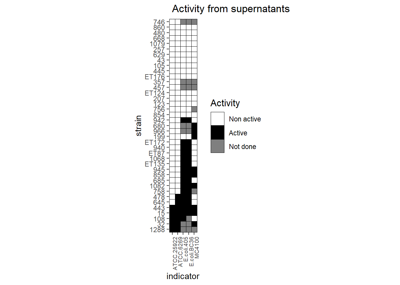
Heatmap format 2
Here you will notice that the Y axis is reverted, in my case I prefer to have the strain 1288 on top of the Y axis so I just add another layer to invert it.
ggplot(tab_tm, aes(indicator, strain)) + geom_tile(aes(fill = factor(value)), colour = "black") + theme(legend.title=element_text(colour = "black", size = 12), axis.text.x = element_text(angle = 90, hjust=1, size=7)) + labs(title = " ", fill='Activity') + scale_fill_manual(values=c("white", "black", "grey"), labels= c('Non active', 'Active', 'Not done')) + coord_fixed() + scale_y_discrete(limits=rev)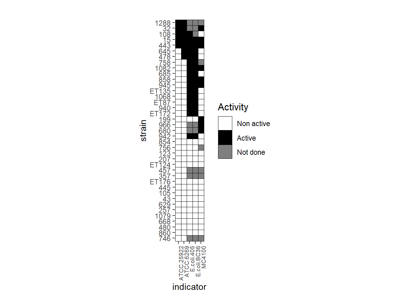
Heatmap Virulence
Loading the packages
Load these packages first
library(reshape)
library(psych)
library(dplyr)
library(data.table)
library(ggplot2)
library(RSelenium)
library(tidyverse)
Import and reformat the Data
Some Errors may Occur, check the class of your data while applying functions, some functions work only on dataframes and some work only on objects of class matrix.
dfv <- read.csv(file = "C:/Users/User/OneDrive - Université Laval/OMICS/Virulence_Analysis/EC41_Virulence_factors__presence_absence.csv")
rownames(dfv) <- dfv[,1] # assign the strains names to the rownames
dfv <- subset (dfv, select = -X) # Remove the column "-X" containing the strains names
dfv_t <- t(dfv) #transpose
rownames(dfv_t) <- colnames(dfv)
colnames(dfv_t) <- rownames(dfv)
dfv_t <- as.data.frame(dfv_t) %>% select("1288_S1", "32_S2", "108_S3", "15_S4", "443_S5", "645_S6", "478_S7", "758_S8", "1082_S9", "685_S10", "858_S11", "945_S12", "ET135_S13", "1068_S14", "ET87_S15", "940_S16", "ET172_S17", "199_S18", "966_S19", "680_S20", "942_S21", "854_S22", "756_S23", "123_S24", "207_S25", "ET124_S26", "457_S27", "357_S28", "ET176_S29", "445_S30", "105_S31", "43_S32", "629_S33", "257_S34", "1079_S35", "668_S36", "480_S37", "860_S38", "746_S39",  "BC36_S40", "Kp405_S41")   # reorder the data in that order
dfv_t$FV <- row.names(dfv_t)
dfv_tm <- melt(dfv_t)                          #Reshape package
colnames(dfv_tm) <- c("FV","Strain","value")
Draw the Plot
preferred.order <- c("1288_S1", "32_S2", "108_S3", "15_S4", "443_S5", "645_S6", "478_S7", "758_S8", "1082_S9", "685_S10", "858_S11", "945_S12", "ET135_S13", "1068_S14", "ET87_S15", "940_S16", "ET172_S17", "199_S18", "966_S19", "680_S20", "942_S21", "854_S22", "756_S23", "123_S24", "207_S25", "ET124_S26", "457_S27", "357_S28", "ET176_S29", "445_S30", "105_S31", "43_S32", "629_S33", "257_S34", "1079_S35", "668_S36", "480_S37", "860_S38", "746_S39",  "BC36_S40", "Kp405_S41")
ggplot(dfv_tm, aes(x=FV, y= factor(Strain, levels = preferred.order))) + geom_tile(aes(fill = factor(value)), colour = "white") + theme(legend.title=element_text(colour = "black", size = 12), axis.text.x = element_text(angle = 90, hjust=1, size=6)) + labs(title="Virulome", size = 15) + labs(x="Virulence factor",y="Strain") + labs(fill='Genotype') + scale_fill_manual(values=c("white", "black"), labels= c('Absence', 'Presence')) + scale_y_discrete(limits=rev) 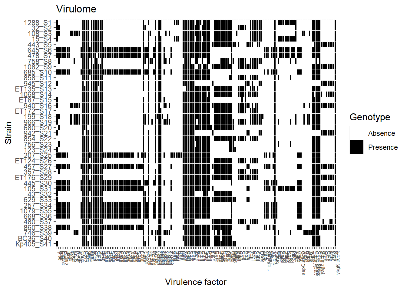
Description of the table
Get some stats such
#describe(dfv)
descri <- describe(dfv)
moyenne <- subset (descri, select = "mean")
moyenne$FV <- row.names(moyenne)
view(moyenne)
Reorder Virulence Factors By Means
moyenne <- moyenne[order(moyenne$mean), ]
good.order<-moyenne$FV
ggplot(moyenne, aes(x = factor(FV, levels = good.order), mean)) + geom_col() 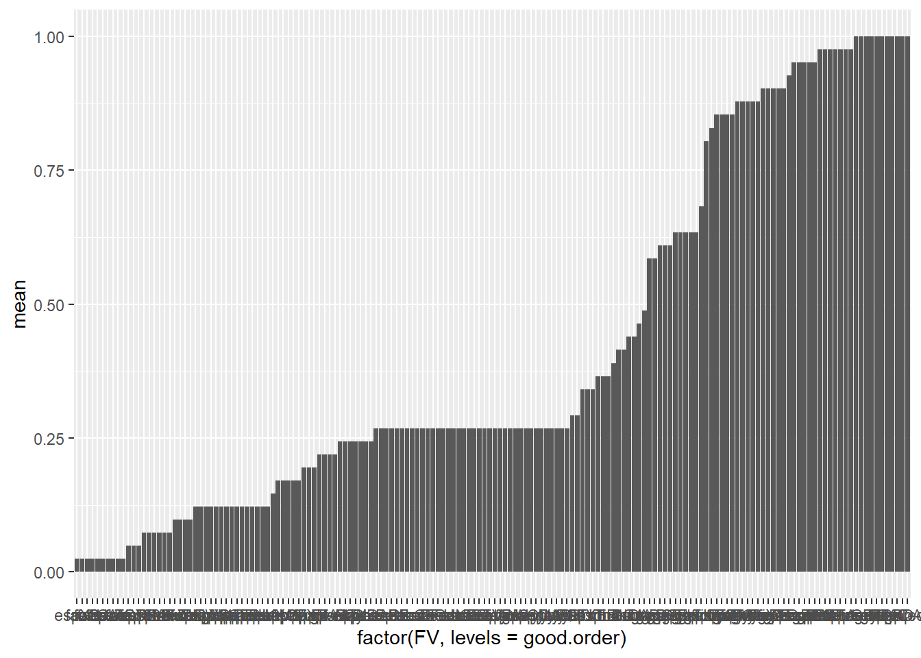
Resistance Phenotype
Our goal here is to visualize the resistance phenotype of the strains of our collections by assigninging the colour red to resistant strains and green to sensitive ones.
We could also assign a colour for the intermediate resistance profile, but it wont be the case here
Import Data
All_df <- read.csv(file = "C:/Users/User/OneDrive - Université Laval/OMICS/Paillasse/All_Data - Copy.csv") # This file contains most of the genomic data
which(colnames(All_df) == "AM") # 306
## [1] 306which(colnames(All_df) == "Col") #322## [1] 322df<- subset(All_df, select = c(306:322)) # I took only the columns related the antibiotic resistance profile
rownames(df) <- All_df$gene # giving my rows relevant names
df_t <- t(df) # transpose my table
rownames(df_t) <- colnames(df)
colnames(df_t) <- rownames(df)
df_t <- as.data.frame(df_t) %>% select("1288_S1", "32_S2", "108_S3", "15_S4", "443_S5", "645_S6", "478_S7", "758_S8", "1082_S9", "685_S10", "858_S11", "945_S12", "ET135_S13", "1068_S14", "ET87_S15", "940_S16", "ET172_S17", "199_S18", "966_S19", "680_S20", "942_S21", "854_S22", "756_S23", "123_S24", "207_S25", "ET124_S26", "457_S27", "357_S28", "ET176_S29", "445_S30", "105_S31", "43_S32", "629_S33", "257_S34", "1079_S35", "668_S36", "480_S37", "860_S38", "746_S39") # reorder my columns in that order
df_t<- df_t[colSums(!is.na(df_t)) > 0] # remove columns that have NA in it
df_t$ATB <- row.names(df_t) # creating "ATB" column, necessary for the melt() to work
df_tm <- melt(df_t) #Reshape package
colnames(df_tm) <- c("ATB","Strain","value") # giving relevant names to the melted table
df_tm$ATB <- factor(df_tm$ATB, levels = c("AM", "AMC", "FEP", "CTX", "FOX", "CAZ", "ATM", "ETP", "CIP", "NA.", "SXT", "C", "TE", "GM", "K", "S", "Col"))
ggplot(df_tm, aes(ATB, Strain)) + geom_tile(aes(fill = factor(value), colour = c("red","green",white) ), colour = "white") + theme(legend.title=element_text(colour = "black", size = 12), axis.text.x = element_text(angle = 45, hjust=1, size=8)) + labs(title="Antibiotic resistance Profile", size = 15) + labs(x="Antibiotic",y="strain") + labs(fill='Phenotype') + scale_fill_manual(values=c("green","red", "red"), labels= c('Sensitive', 'Resistant', 'Resistant'))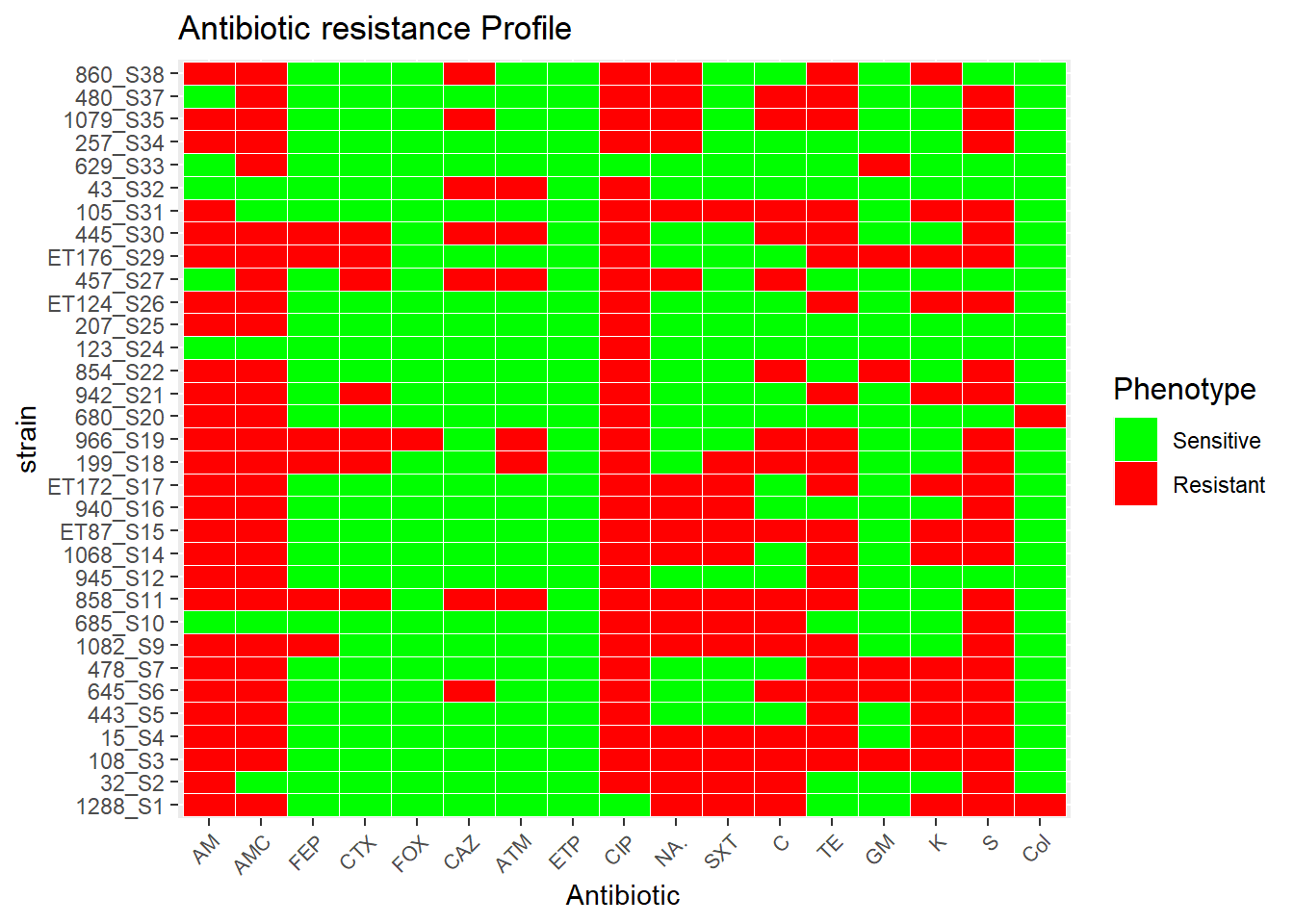
Resistance Heatmap
Loading the necessary packages
library(reshape)
library(psych)
library(dplyr)
library(data.table)
library(ggplot2)
library(RSelenium)
library(ggplot2)
Importing and transforming data
R_Genes <- read.csv(file = "C:/Users/User/OneDrive - Université Laval/OMICS/Résistance_Analyse/R_Genes.csv" )

rownames(R_Genes) <- R_Genes$gene

R_Genes <- subset(R_Genes, select = -c(1))

R_Genes <- subset(R_Genes, select=-c(which(colnames(R_Genes)=="BC36_S40"))) # Remove this sample

R_Genes <- subset(R_Genes, select=-c(which(colnames(R_Genes)=="Kp405_S41"))) # Remove this sample


R_Genes_t <- t(R_Genes)

R_Genes_tm <- reshape2::melt(R_Genes_t)

colnames(R_Genes_tm) <- c("strain","gene","value")

p<-ggplot(R_Genes_tm, aes(strain, gene)) + geom_tile(aes(fill = factor(value)), colour = "black") + theme(legend.title=element_text(colour = "black", size = 3), axis.text.x = element_text(angle = 90, hjust=1, size=9), axis.text.y = element_text(size = 3.5)) + labs(title="Resistomes", size = 100) + labs(x="Strains",y="Resistance genes and mutations") + labs(fill=' ', ) + scale_fill_manual(values=c("black", "red", "green"), labels= c('Absence', 'strict hit', 'perfect hit'))

p #view plot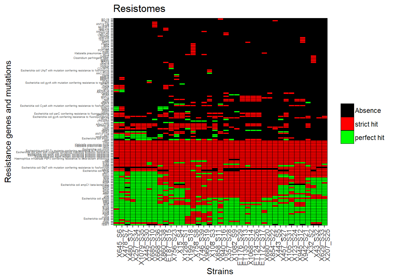
Saving the plot
ggsave(p, path = "C:/Users/User/OneDrive - Université Laval/Article Drafts/1st article Tables and Figures/", filename = "heatmap.pdf")Changing the order of the strains
We want to put a custom order before redrawing the graph
good_order <- c("X1288_S1","X32_S2","X108_S3","X15_S4","X443_S5","X645_S6","X478_S7","X758_S8","X1082_S9","X685_S10","X858_S11","X945_S12","ET135_S13","X1068_S14","ET87_S15","X940_S16","ET172_S17","X199_S18","X966_S19","X680_S20","X942_S21","X854_S22","X756_S23","X123_S24","X207_S25","ET124_S26","X457_S27","X357_S28","ET176_S29","X445_S30","X105_S31","X43_S32","X629_S33","X257_S34","X1079_S35","X668_S36","X480_S37","X860_S38","X746_S39")

p1<-ggplot(R_Genes_tm, aes(x=factor(strain, levels = good_order ), gene)) + geom_tile(aes(fill = factor(value)), colour = "black") + theme(legend.title=element_text(colour = "black", size = 3), axis.text.x = element_text(angle = 90, hjust=1, size=9), axis.text.y = element_text(size = 3.5)) + labs(title="Resistomes", size = 100) + labs(x="Strains",y="Resistance genes and mutations") + labs(fill=' ', ) + scale_fill_manual(values=c("black", "red", "green"), labels= c('Absence', 'strict hit', 'perfect hit'))

p1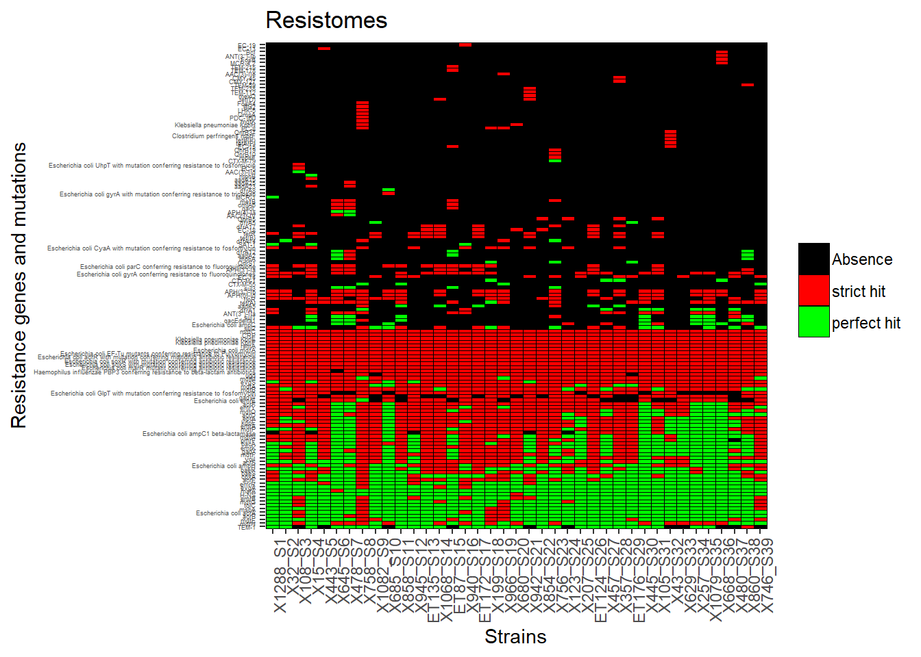
Get the genotype from this data
In the previous code we have been able to draw a heatmap of the strains. In the case that i want to have the Profile of each strain I have to proceed as following.
Load the data and subset the Antibiotic resistance profile section
All_df <- read.csv(file = "C:/Users/User/OneDrive - Université Laval/OMICS/Paillasse/All_Data - Copy.csv") # This file contains most of the genomic data
which(colnames(All_df) == "AM") # 306
## [1] 306which(colnames(All_df) == "Col") #322## [1] 322antibiogram<- subset(All_df, select = c(306:322)) # I took only the columns related the antibiotic resistance profile
rownames(antibiogram) <- All_df$gene # giving my rows relevant names
antibiogram<- t(antibiogram)
antibiogram <- antibiogram[, !colSums(is.na(antibiogram)), drop = FALSE]# remove columns that have NA in it
antibiogram<- t(antibiogram)Declaring an empty Dataframe to store results
return_final<-data.frame()Design a for loop
For loop to read into matrix and then fill a new table with the resistance profile
The following lines will :
Read the table line by line with a first for loop. each line (strain) will be assigned to a temporary table “tmp”.
Subset only the columns (antibiotics) that have a value equal to 1 (resistant phenotype) and assign it to another temporary table “tmp1”.
Declare an empty string vector here called “profile”.
Fill the empty vector with the column names of the table “tmp1” that contains only column names of antibiotics to which a strain is resistant.
Fill a temporary table with the results.
Bind all the temporary tables into a final results table
data <- as.data.frame(antibiogram)
for (i in row.names(data)) {
  tmp<-data[c(i),]
  tmp1 <- subset(tmp, select = c(tmp==1))
  nbr<- print(length(tmp1))
  profile<-as.character(" ")
  for (j in colnames(tmp1)){
    profile<- paste0(profile,"/", print(j))
  }
  return_tmp <- data.frame("Strain" = i, "profile" = profile, "Resistant to" = nbr, stringsAsFactors = F)
  return_final<-rbind(return_final, return_tmp)
}
View the Results
view(return_final)Save the results in a csv table
In order to keep these results
write.csv(return_final, file = "/Users/User/OneDrive - Université Laval/OMICS/Paillasse/Antibiogramme_profile.csv" )Description for a table
table <- describe(df)
view(table)
ggplot(table, aes(x=vars, y=mean)) + geom_bar(stat = 'identity')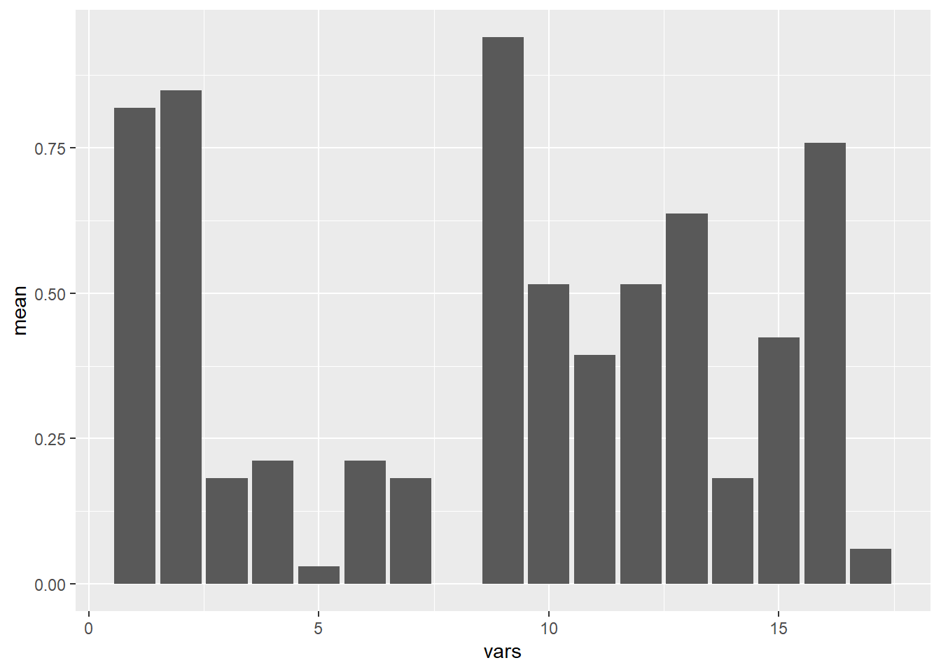
#Mapping samples origins
I want to show where my samples come from on a map
Load necessary packages
library(leaflet)
library(tmaptools)
Preparing Data
Im going to try to take GPS localisation of the samples. Try to give them different names according to the names in this server https://nominatim.openstreetmap.org/
Rendering the map
simple<- data.frame("Samples"=preferred.order, ID= c("Nabeul", "ksour essef", "mellassine", "bou merdes", "sidi bou ali", "kemicha", "grombalia", "Gouvernorat Siliana", "Jandouba", "Gouvernorat Monastir", "Chela", "Sijoumi", "Sfax", "Mahres", "Stade Municipal Menzel Chaker", "El Habibia", "Manouba", "La Marsa", "تونس العاصمة" , "Municipalité De Beb Lakwes", "Bizerte", "Chela", "El Aouina", "mellassine", "Gouvernorat Béja", "Zaghouan", "Bir Ali Ben Khalifa", "Chela","Gouvernorat Mahdia", "Hayy Ibn Khaldun", "mellassine", "Délégation Ksour Essef", "تونس العاصمة", "Rue Ibn Charaf", "Intilaka", "Rue Touhami Amar", "Agareb", "Aïn Draham", "Rue Beb Jdid", NA, NA))
cities<- simple$ID[1:39] # cut the names of the cities and remove the last values which are NAs
query <- geocode_OSM(cities)
m <- leaflet() %>%
     addTiles(urlTemplate = "https://{s}.tile.openstreetmap.org/{z}/{x}/{y}.png") %>%    addMarkers(query$lon, query$lat, label = query$query,  icon = makeIcon(iconUrl ="https://fanblairfarm.co.uk/wp-content/uploads/2020/11/chicken-icon-2.png", iconWidth = 17, iconHeight= 17))
Try this format
m %>% addProviderTiles(providers$MtbMap) %>%
  addProviderTiles(providers$Stamen.TonerLines,
    options = providerTileOptions(opacity = 0.35)) %>%
  addProviderTiles(providers$Stamen.TonerLabels)
Best map until now
#Red chicken Tile, the best one until now

m <- leaflet() %>%
    addTiles(urlTemplate = "https://{s}.tile.openstreetmap.org/{z}/{x}/{y}.png") %>%    addMarkers(query$lon, query$lat, label = query$query,  icon = makeIcon(iconUrl ="https://www.downloadclipart.net/large/chicken-png-transparent-image.png", iconWidth = 17, iconHeight= 17))

m %>% addProviderTiles(providers$Stamen.TonerLite) #best map until now
Make PCA for my data
I will find this usefull to interprete my data, the thing is some of the vectors here were manually typed
Loading Libraries
library(logisticPCA)
library(ggplot2)
Importing the Data and rendering the graph
All_df <- read.csv(file = "C:/Users/User/OneDrive - Université Laval/OMICS/Paillasse/All_Data - Copy.csv") # This file contains most of the genomic data
data<- subset(All_df, select = c(-gene))
Activity <-c(rep("Active", 21), rep("Inactive", 18))

data <- as.matrix(data) # with matrix you can have repetitive rownames
rownames(data)<- Activity
logsvd_model = logisticSVD(data, k = 2)
logsvd_model
## 39 rows and 321 columns
## Rank 2 solution
##
## 53.8% of deviance explained
## 470 iterations to convergelogpca_cv = cv.lpca(data, ks = 2, ms = 1:10)
plot(logpca_cv)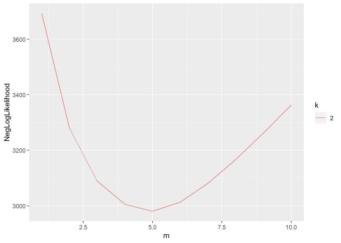
logpca_model = logisticPCA(data, k = 2, m = which.min(logpca_cv))
plot(logsvd_model, type = "trace")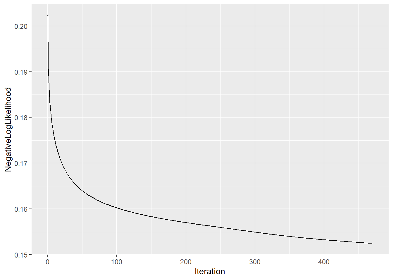
Activity<- rownames(data)
plot(logpca_model, type = "scores") + geom_point(aes(colour = Activity)) +
ggtitle("Logistic PCA") + scale_colour_manual(values = c("blue", "red")) 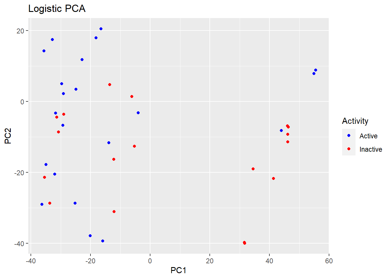
plot(logsvd_model, type = "scores") + geom_point(aes(colour = Activity)) + ggtitle("Exponential Family PCA") + scale_colour_manual(values = c("blue", "red"))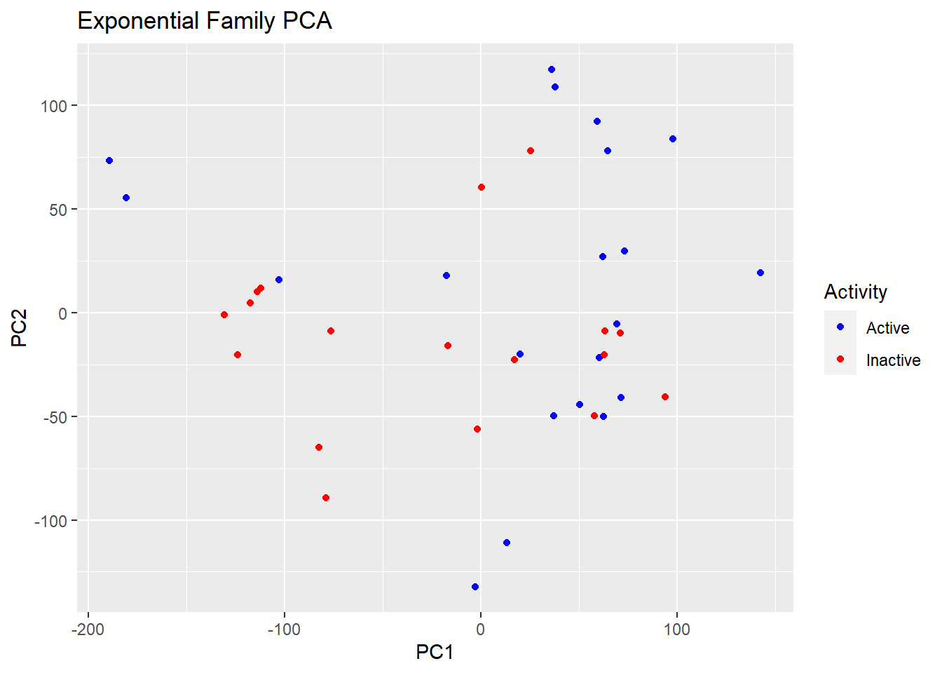
PCA coloration depending on the criteria of bacteriocin Production
Here we will use the same model, the coordinates of the population will stay in the same place no need to redo the calculation. However we will colour the strains depending on the criterium of bacteriocin production
Mcc <- c("J25", "J25+C7+colV", "J25+colV", "J25", "J25+colV", "inactive", "inactive", "inactive", "colV", "inactive", "C7+colV", "colV", "inactive", "colV", "inactive", "colV", "colV", "inactive", "colV", "inactive", "inactive", "colV", rep("inactive", 5), rep("colV", 2), rep("inactive", 7), "colV", "inactive", "inactive")
Mcc[Mcc=="inactive"] <- "Non-producer"
Mcc[Mcc!="Non-producer"] <- "Bacteriocin producer"


plot(logsvd_model, type = "scores") + geom_point(aes(colour = Mcc)) +
  ggtitle("Exponential Family PCA") + scale_colour_manual(values = c("blue", "orange"))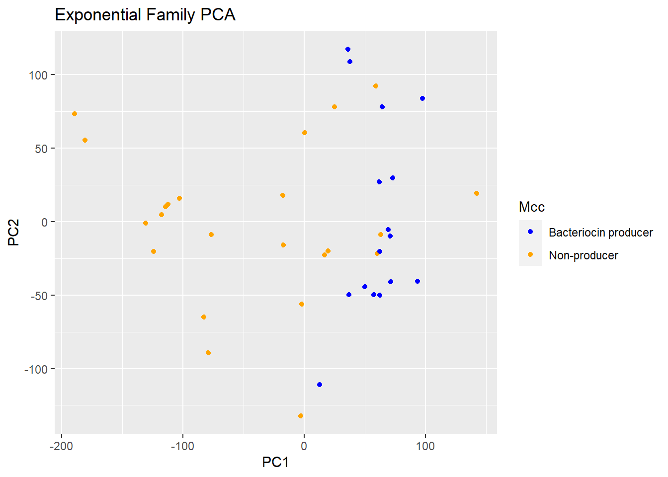
p1 <- plot(logpca_model, type = "scores") + geom_point(aes(colour = Mcc)) +   ggtitle("Logistic PCA") + scale_colour_manual(values = c("blue", "orange"))

p1 #visualize the plot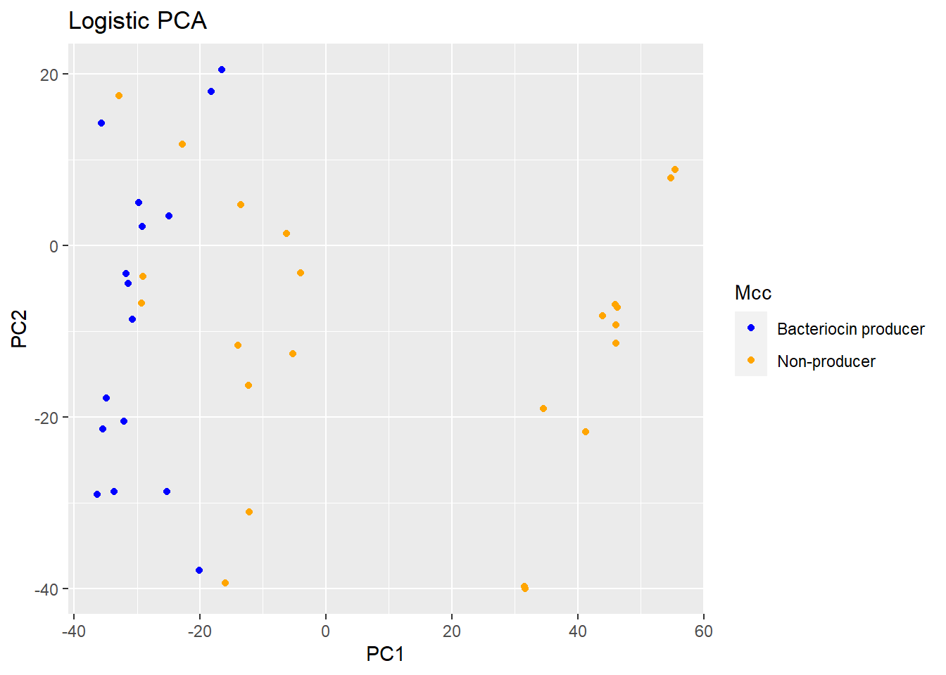
PCA depending on the degree of Virulence
Same thing but different colours depending on the pathotype.
#Virulence<- dput(as.character(clipr::read_clip())) # very useful to copy paste a vector

Virulence<- c("APEC potential", "APEC", "APEC potential", "APEC potential", "APEC potential", "AFEC", "AFEC", "APEC", "APEC", "APEC potential", "APEC", "APEC potential", "APEC", "APEC", "APEC potential", "APEC", "APEC", "APEC potential", "APEC", "APEC potential", "APEC potential", "APEC", "APEC potential", "AFEC", "AFEC", "APEC", "AFEC", "APEC", "APEC", "AFEC", "AFEC", "AFEC", "AFEC", "AFEC", "AFEC", "AFEC",
"APEC", "AFEC", "APEC potential")

plot(logsvd_model, type = "scores") + geom_point(aes(colour = Virulence)) +
  ggtitle("Exponential Family PCA") + scale_colour_manual(values = c("green", "red", "purple"))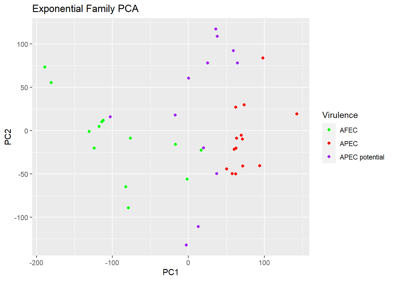
p2 <- plot(logpca_model, type = "scores") + geom_point(aes(colour = Virulence)) +
  ggtitle("Logistic PCA") + scale_colour_manual(values = c("green", "red", "purple"))

p2 #visualize the plot 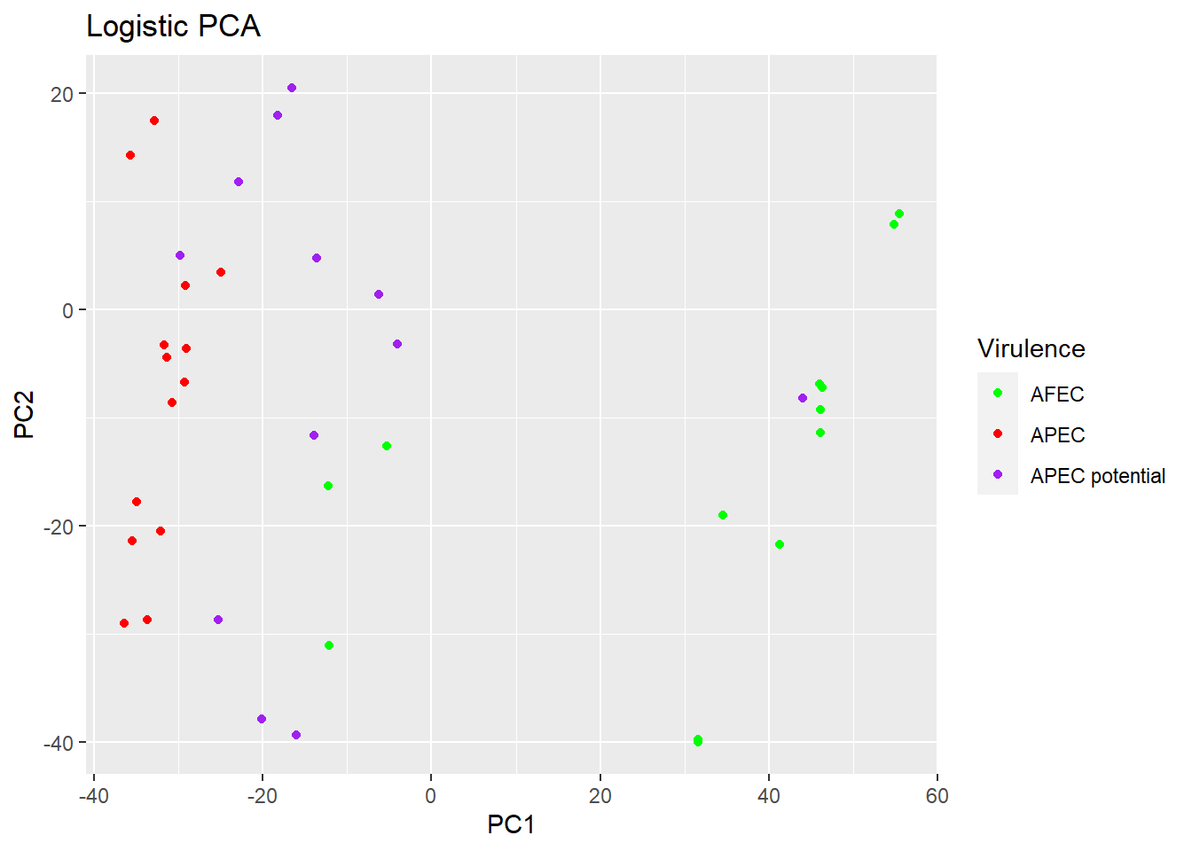
PCA depending on Phylogroup
#Phylogroup <- dput(as.character(clipr::read_clip()))
Phylogroup <- c("A", "A", "F", "A", "B1", "A", "A", "B1", "B1", "A", "B1", "A", "B1", "B1", "A", "F", "B1", "B2", "D", "B1", "A", "B1", "B1", "A", "A", "B1", "A", "B1", "B1", "A", "A", "A", "A", "A", "A", "A", "A", "A", "D")

plot(logsvd_model, type = "scores") + geom_point(aes(colour = Phylogroup)) +   ggtitle("Exponential Family PCA") + scale_colour_manual(values = c("green", "red", "purple", "yellow", "grey"))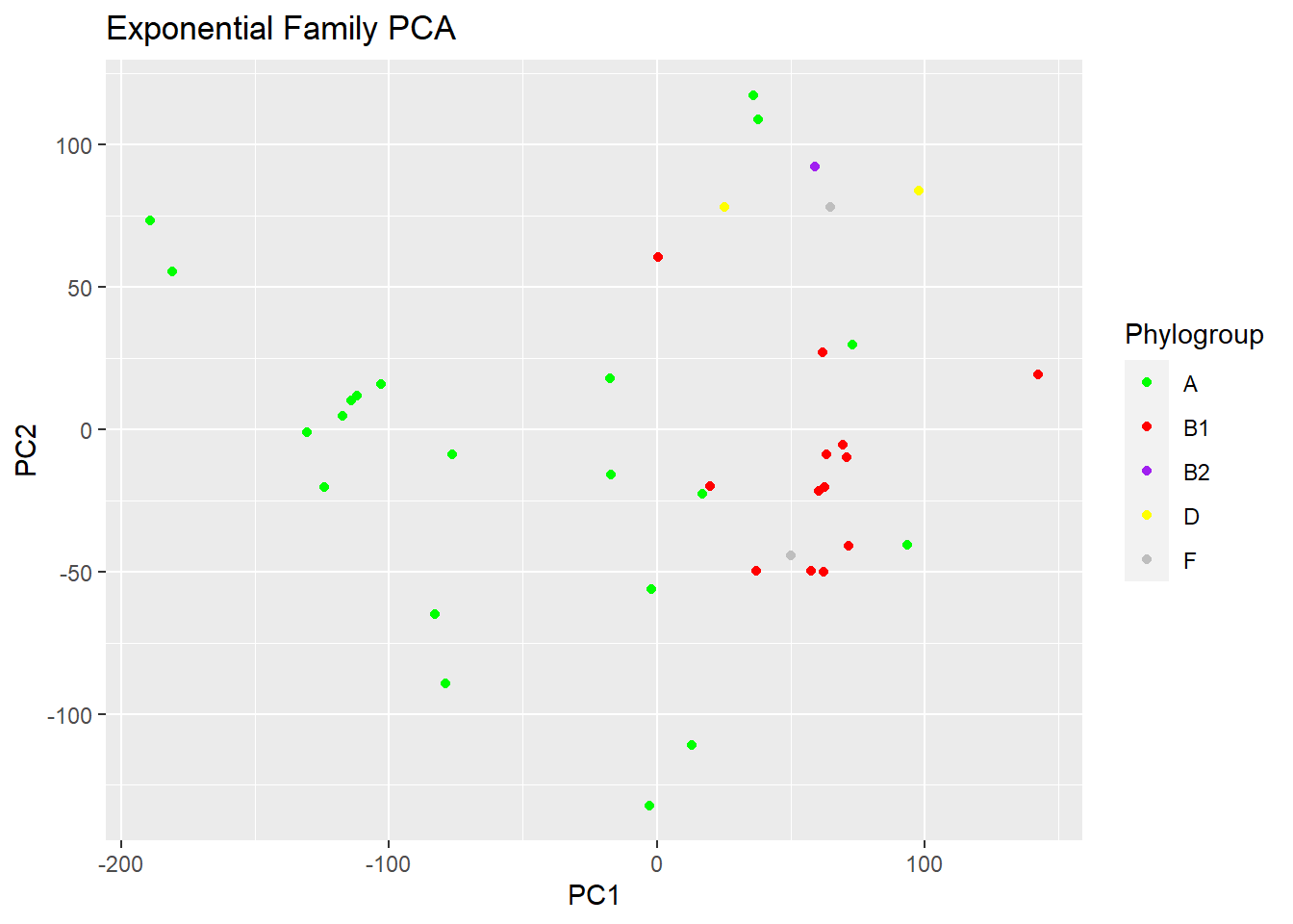
p3 <- plot(logpca_model, type = "scores") + geom_point(aes(colour = Phylogroup)) +   ggtitle("Logistic PCA") + scale_colour_manual(values = c("green", "red", "purple", "yellow", "grey"))

p3 # visualize the plot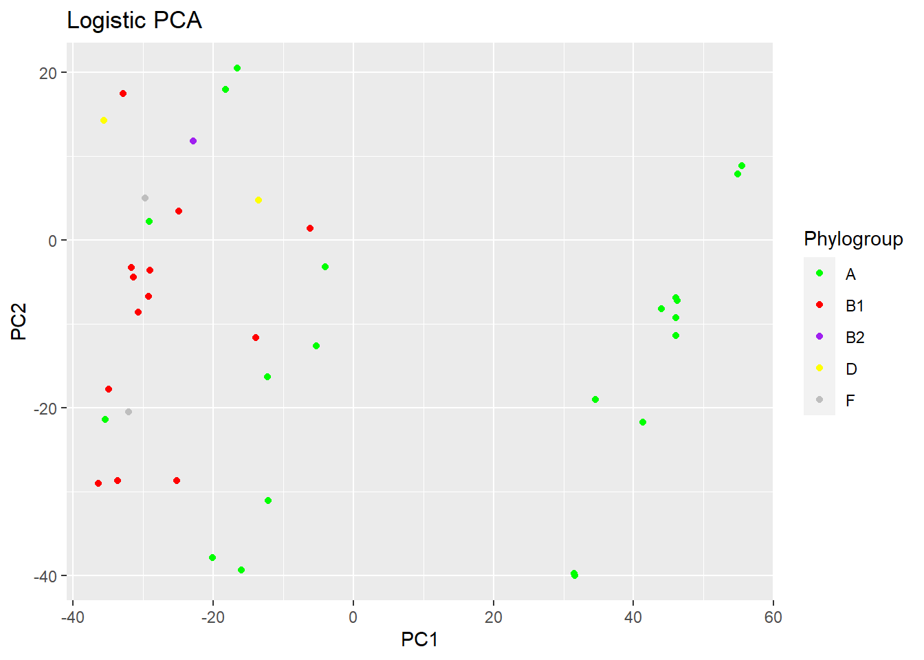
#Merging the plots
Loadin the Patchwork package
library(patchwork)
p1+p2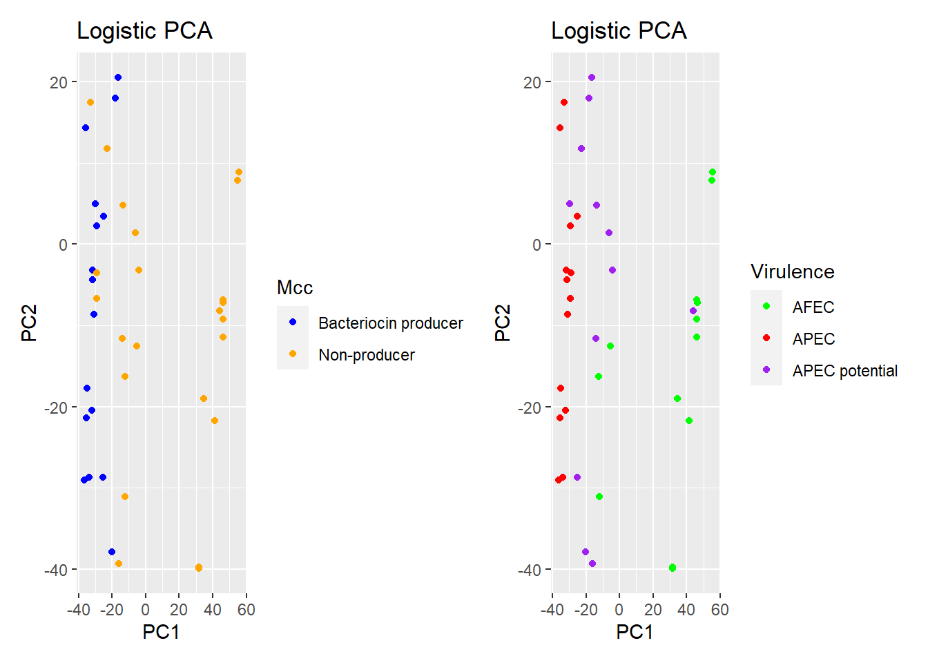
Usefull stuff
merging two tables by their ID
Let’s suppose that we have two tables that contain the same unique IDs, this function is usefull to merge the two tables depending on these IDs even if the rows are not ordered. Here we merge two tables data1 and data2 by their ID names
merge(x= data1, y=data2, by= "ID", all=TRUE)Replace all NA’s with 0 in a dataframe
Here we replace all the NAs in a data by zero, easy stuff
data[is.na(data)] <- 0Calculate correlation for binary table
Here i want to calculate the pearson’s correlation coefficient between my different variables. By checking the bibliography, the cor() function should do the work. If there is a variable that takes the value 1 or 0 across all the population, we will see this Warning message : In cor(data) : the standard deviation is zero We can make a heatmap Based on that using the pheatmap package
cor_data <- cor(data)
library(pheatmap)
cor_data[is.na(cor_data)] <- 0
pheatmap::pheatmap(cor_data)
Plasmids
So I have a Table containing some presence/absence Data of some plasmids across my genomes.
Import Data
The First time that I worked with my data, i just used clipr package to get it from the clipboard, then i saved it to a file that i will read the second time.
#tb2 <-clipr::read_clip_tbl(header=TRUE)

#write.csv(tb2 , row.names = FALSE, file = "C:/Users/User/OneDrive - Université Laval/OMICS/Paillasse/Plasmids_binary.csv")

tb2 <- read.csv(file = "C:/Users/User/OneDrive - Université Laval/OMICS/Paillasse/Plasmids_binary.csv")
Replace NAs
It’s as easy as this
tb2[is.na(tb2)== TRUE]<-0Phylogenetic Tree
Load ape Package
library(ape)Import newick file
mytree<-read.tree("C:/Users/User/OneDrive - Université Laval/OMICS/Paillasse/tree.newick.txt")

mytree$tip.label # to check the edge number of the APEC strain
## [1] "Sample36"
## [2] "Sample34"
## [3] "Sample30"
## [4] "Sample35"
## [5] "Sample10"
## [6] "Sample7"
## [7] "Sample6"
## [8] "Sample2"
## [9] "Sample4"
## [10] "Sample1"
## [11] "Sample31"
## [12] "Sample27"
## [13] "Sample38"
## [14] "Sample21"
## [15] "Sample12"
## [16] "Sample37"
## [17] "Sample25"
## [18] "Sample33"
## [19] "Sample32"
## [20] "Sample15"
## [21] "Sample24"
## [22] "Sample41"
## [23] "NC_000913_3_Escherichia_coli_str_K_12_substr_MG1655_fixed"
## [24] "Sample14"
## [25] "Sample13"
## [26] "Sample17"
## [27] "Sample26"
## [28] "Sample23"
## [29] "Sample11"
## [30] "Sample20"
## [31] "Sample22"
## [32] "Sample40"
## [33] "NC_020163_1_Escherichia_coli_APEC_O78_fixed"
## [34] "NC_018658_1_Escherichia_coli_O104_H4_str_2011C_3493_fixed"
## [35] "Sample9"
## [36] "Sample29"
## [37] "Sample5"
## [38] "Sample28"
## [39] "Sample8"
## [40] "Sample18"
## [41] "NC_017634_1_Escherichia_coli_O83_H1_str_NRG_857C_fixed"
## [42] "Sample3"
## [43] "Sample16"
## [44] "NC_011750_1_Escherichia_coli_IAI39_fixed"
## [45] "Sample19"
## [46] "CU928163_2_Escherichia_coli_UMN026_fixed"
## [47] "Sample39"
## [48] "NC_002695_2_Escherichia_coli_O157_H7_str_Sakai_fixed"rerootTree<- root(mytree, mytree$tip.label[33])
rerootTree$tip.label ## [1] "Sample36"
## [2] "Sample34"
## [3] "Sample30"
## [4] "Sample35"
## [5] "Sample10"
## [6] "Sample7"
## [7] "Sample6"
## [8] "Sample2"
## [9] "Sample4"
## [10] "Sample1"
## [11] "Sample31"
## [12] "Sample27"
## [13] "Sample38"
## [14] "Sample21"
## [15] "Sample12"
## [16] "Sample37"
## [17] "Sample25"
## [18] "Sample33"
## [19] "Sample32"
## [20] "Sample15"
## [21] "Sample24"
## [22] "Sample41"
## [23] "NC_000913_3_Escherichia_coli_str_K_12_substr_MG1655_fixed"
## [24] "Sample14"
## [25] "Sample13"
## [26] "Sample17"
## [27] "Sample26"
## [28] "Sample23"
## [29] "Sample11"
## [30] "Sample20"
## [31] "Sample22"
## [32] "Sample40"
## [33] "NC_020163_1_Escherichia_coli_APEC_O78_fixed"
## [34] "NC_018658_1_Escherichia_coli_O104_H4_str_2011C_3493_fixed"
## [35] "Sample9"
## [36] "Sample29"
## [37] "Sample5"
## [38] "Sample28"
## [39] "Sample8"
## [40] "Sample18"
## [41] "NC_017634_1_Escherichia_coli_O83_H1_str_NRG_857C_fixed"
## [42] "Sample3"
## [43] "Sample16"
## [44] "NC_011750_1_Escherichia_coli_IAI39_fixed"
## [45] "Sample19"
## [46] "CU928163_2_Escherichia_coli_UMN026_fixed"
## [47] "Sample39"
## [48] "NC_002695_2_Escherichia_coli_O157_H7_str_Sakai_fixed"plot(rerootTree)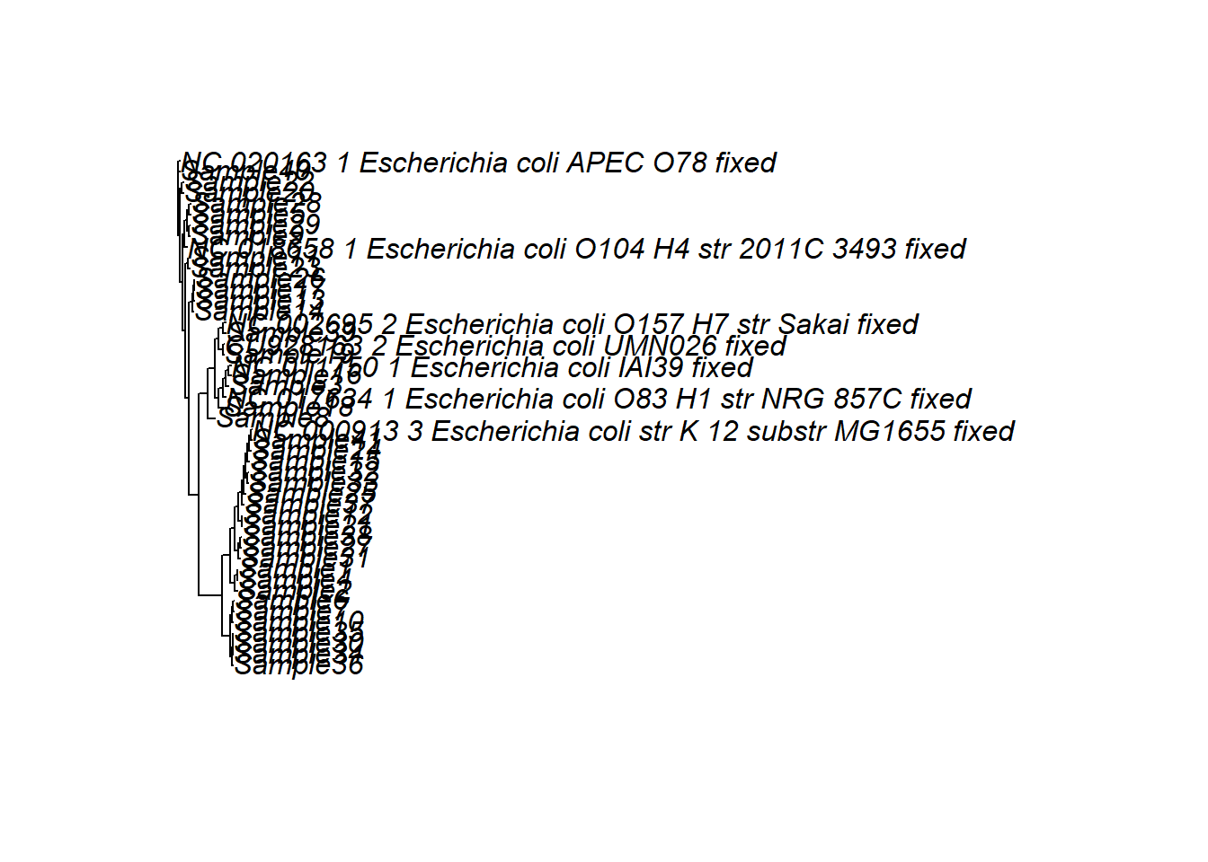
edgecol<- vector()
edgecol[1:41] = "black"

tipcol<- vector()
tipcol[1:41] = "black"

arbre <- plot.phylo(rerootTree, "tidy", main= "phylogenetic analysis based on Average nucleotide identity", edge.color = edgecol, cex = 0.6 , tip.color = tipcol, use.edge.length = FALSE, x.lim = 90) 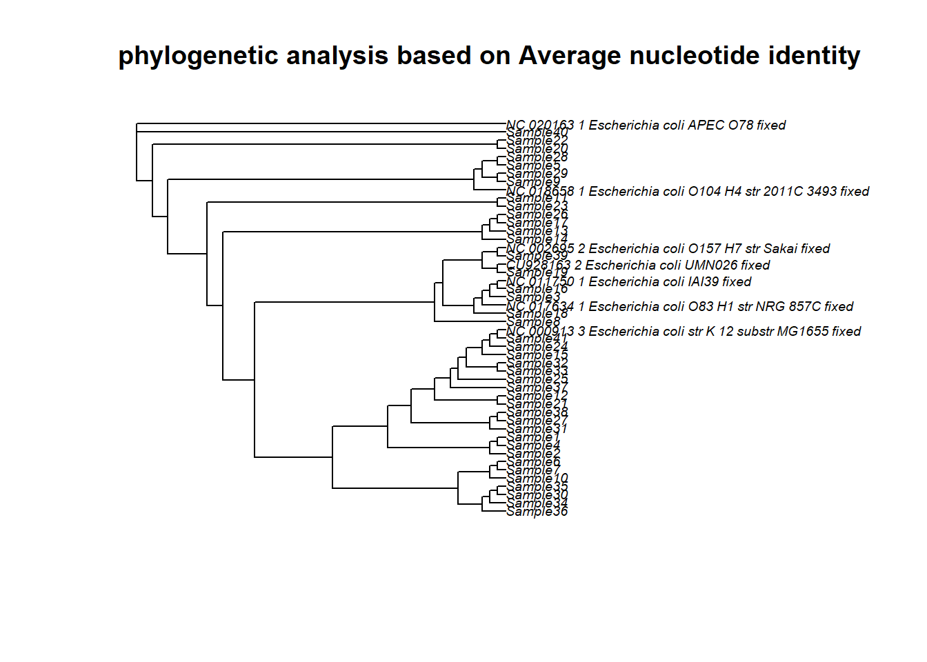
Adding labels (optionnal)
#edgelabels(font=0.5, cex=0.5)
#tiplabels(font=0.05, cex=0.5)
Chi Square test on binary data
credit goes to https://stackoverflow.com/questions/71666349/multiple-chi-square-tests-in-r
data <- read.csv(file = "C:/Users/User/OneDrive - Université Laval/OMICS/Paillasse/All_Data - Copy.csv", stringsAsFactors = TRUE) # This file contains most of the genomic data

# Identify columns with only one level as a value
cols_to_remove <- sapply(data, function(x) length(unique(x)) == 1)

#Remove columns with only one level as a value
data <- data[, !cols_to_remove]

# Split the data into response (sample) and predictor (parameter) variables
#response <- data[,1]
#predictors <- data[,2:ncol(data)]

#response <- as.factor(response) #necesary for chisq.test to work

# Use the chi-squared test to determine the association between each parameter
chi_sq_test <- data %>%
    select(-gene) %>%
    colnames() %>%
    combn(2) %>%
    t() %>%
    as_tibble() %>%
    rowwise %>%
    mutate(chisq_test = list(
        table(data[[V1]], data[[V2]]) %>% chisq.test()
    ),
    chisq_pval = chisq_test$p.value
    )

# Sort the chi-squared test statistics in descending order to determine the most discriminatory parameters
sorted_chi_sq_test <- chi_sq_test[order(chi_sq_test$chisq_pval, decreasing = FALSE), ]

# Identify the top 10 most discriminatory parameters
top_10_params <- head(sorted_chi_sq_test, 10)

# Print the top 10 most discriminatory parameters
print(top_10_params)
## # A tibble: 10 × 4
## # Rowwise:
## V1 V2 chisq_test chisq_pval
## <chr> <chr> <list> <dbl>
## 1 APH.6..Id APH.3....Ib <htest> 0.00000000316
## 2 gspC gspE <htest> 0.00000000334
## 3 gspC gspF <htest> 0.00000000334
## 4 gspE gspF <htest> 0.00000000334
## 5 gspH gspI <htest> 0.00000000349
## 6 gspH gspJ <htest> 0.00000000349
## 7 gspH gspK <htest> 0.00000000349
## 8 gspI gspJ <htest> 0.00000000349
## 9 gspI gspK <htest> 0.00000000349
## 10 gspJ gspK <htest> 0.00000000349Download Data from NCBI
Here I want to download data about all the prokaryotic genomes in NCBI. Use the option -O to name the output file.
cd /mnt/c/Users/User/OneDrive - Université Laval/OMICS/Ref

wget "https://ftp.ncbi.nlm.nih.gov/genomes/GENOME_REPORTS/prokaryotes.txt" -O prokaryotes_20230515.txt
Count number of Genomes of Escherichia coli
grep -c "Escherichia coli" prokaryotes_20230515.txtCreate a file containing only Data about Escherichia coli
head -n 1 prokaryotes_20230515.txt  > Escherichia_coli_20230515.txt # first get the column names

 grep "Escherichia coli" prokaryotes_20230515.txt >> Escherichia_coli_20230515.txt # get the lines that contain Escherichia coli and redirect it to the file that we just created
In that file, the column number 19 has the accession numbers, we can check that by typing this command
cut -f 19 -d " " Escherichia_coli_20230515.txt | head -n 1To get the metadata for these genomes, there is a special tool for that that makes it easy. We need to install it using conda as described here https://www.ncbi.nlm.nih.gov/datasets/docs/v1/download-and-install/
Getting metadata for a genome assembly is as easy as this
datasets summary genome accession GCA_024300685.1 > test_delete.json

jq . test_delete.json | head --lines=10  # better visualize a json file
for some reason This didnt work, so I ll just download one genome to try.
datasets download genome accession GCF_003018795.1 --filename testini.zip # download genome data package
dataformat tsv genome --inputfile testini/ncbi_dataset/data/assembly_data_report.jsonl
With the previous code, I managed to download metadata with a forloop
for accession in $(cut -f 19 -d " " Escherichia_coli_20230515.txt | tail -n+2); do echo $accession ; done
Create a folder, download data reports, unzip them, format the json reports of the genomes and redirect to the file metadata.tsv in parent directory, finish by deleting genome data fromn the download folder
mkdir download && cd download && for accession in $(cut -f 19 -d " " ../Escherichia_coli_20230515.txt | tail -n+2); do echo "downloading data for $accession" && datasets download genome accession $accession --filename $accession.zip && unzip $accession.zip -d $accession && echo "extraction done" && dataformat tsv genome --inputfile ${accession}/ncbi_dataset/data/assembly_data_report.jsonl >> ../metadata.tsv && rm -r GCA* && echo "files removed" ; done cd ..
grep all the lines that contain unique accession numbers in the metadata, -t option for the sort command defines the delimitor
head -n+1 metadata.tsv  > metadata_APEC.tsv

grep APEC metadata.tsv | sort -t "    " -u -k 50,50 | sort -t "       " -u -k 21,21  >> metadata_APEC.tsv # the column 50 has the accession numbers and the column 21  has the project numbers

tail -n+2  metadata_APEC.tsv | wc -l # counting the number of strains from different projects, 17 APEC strains
Search for unique assemblies of commensal Escherichia coli strains isolated form Poultry
grep -i 'poultry\|broiler\|chicken' metadata.tsv | grep -i 'AFEC\|healthy\|commensal' | sort -t "     " -u -k 21,21  | sort -t "    " -u -k 50,50 | wc -l # there are 6 unique assemblies of commensal E. coli

head -n+1 metadata.tsv  > metadata_6_AFEC.tsv


grep -i 'poultry\|broiler\|chicken' metadata.tsv | grep -i 'AFEC\|healthy\|commensal' | sort -t "     " -u -k 21,21  | sort -t "    " -u -k 50,50 >> metadata_6_AFEC.tsv
Blast for APEC pathotype predictor genes
For the APEC, Im going to confirm their APEC status by local alignment using the 5 Predictor genes for APEC pathotype.
conda activate abricate # activate environment

abricate --setupdb #after adding a fasta file to /path/to/abricate/db/database_name/sequences.fa

cd download/

conda activate ncbi_datasets

for accession in $(tail -n+2 ../metadata_APEC.tsv | cut -f 50); do echo "Downloading data for $accession" && datasets download genome accession $accession --filename $accession.zip && unzip $accession.zip -d $accession && echo "extraction done"; done # Downloading data

conda activate abricate

for accession in $(tail -n+2 ../metadata_APEC.tsv | cut -f 50) ; do wc -l $accession/ncbi_dataset/data/$accession/${accession}*.fna ; done # Testing that th eloop works

for accession in $(tail -n+2 ../metadata_APEC.tsv | cut -f 50) ; do abricate --db APEC $accession/ncbi_dataset/data/$accession/${accession}*.fna  >> ./APEC_blast_${accession}.tsv ; done


abricate --summary ./APEC_blast_*.tsv  > ../APEC_blast_summary.tsv #make a table summary of this

rm -fr *GCA*  # remove all the folders and files from the download folder
Show accession numbers of the strains that contains all the 5 genes
While visualizing the table, some of the Genomes that were reported as APEC, didnt contain all of the 5 predictor genes for the APEC pathotype. The following command line, shows the accession numbers of the strains that have all of the five predictor genes, depending on summary table generated by abricate
awk '$2==5' ../APEC_blast_summary.tsv | awk '{print $1}' | cat | sed 's/.\/APEC_blast_//g' | sed 's/.tsv//g' # 9strains are confirmed APECGet the metadata of the APEC confirmed strains
for accession in $(awk '$2==5' ../APEC_blast_summary.tsv | awk '{print $1}' | cat | sed 's/.\/APEC_blast_//g' | sed 's/.tsv//g'); do echo "$accession is an APEC strain"; done # Testing loop

activate ncbi_datasets
cd downloads/
for accession in $(awk '$2==5' ../APEC_blast_summary.tsv | awk '{print $1}' | cat | sed 's/.\/APEC_blast_//g' | sed 's/.tsv//g'); do echo "downloading data for $accession" && datasets download genome accession $accession --filename $accession.zip && unzip $accession.zip -d $accession && echo "extraction done" && dataformat tsv genome --inputfile ${accession}/ncbi_dataset/data/assembly_data_report.jsonl >> ../metadata_APEC_confirmed.tsv && rm -r GCA* && echo "files removed" ; done && cd ..
Read Antibiogram from excell tables
Read the tables, each table contains the inhibition diameters of a specific strain
t1<- readxl::read_excel("E:/Share_Ubuntu_WGS/Antibiogram_05_2023/746.xlsx")
t2<- readxl::read_excel("E:/Share_Ubuntu_WGS/Antibiogram_05_2023/756.xlsx")
t3<- readxl::read_excel("E:/Share_Ubuntu_WGS/Antibiogram_05_2023/758.xlsx")
t4<- readxl::read_excel("E:/Share_Ubuntu_WGS/Antibiogram_05_2023/357.xlsx")
t5<- readxl::read_excel("E:/Share_Ubuntu_WGS/Antibiogram_05_2023/ET_135.xlsx")
t6<- readxl::read_excel("E:/Share_Ubuntu_WGS/Antibiogram_05_2023/668.xlsx")
Only Keep the two first columns of each table
t1 <- subset(t1, select = c(1,2))
t2 <- subset(t2, select = c(1,2))
t3 <- subset(t3, select = c(1,2))
t4 <- subset(t4, select = c(1,2))
t5 <- subset(t5, select = c(1,2))
t6 <- subset(t6, select = c(1,2))
Change column names
colnames(t1)<- c("Antibiotic", "746_S39")
colnames(t2)<- c("Antibiotic", "756_S23")
colnames(t3)<- c("Antibiotic", "758_S8")
colnames(t4)<- c("Antibiotic", "357_S28")
colnames(t5)<- c("Antibiotic", "ET135_S13")
colnames(t6)<- c("Antibiotic", "668_S36")
Merge Tables
t <- merge(x= t1, y=t2, by= "Antibiotic", all=TRUE)
t <- merge(x= t, y=t3, by= "Antibiotic", all=TRUE)
t <- merge(x= t, y=t4, by= "Antibiotic", all=TRUE)
t <- merge(x= t, y=t5, by= "Antibiotic", all=TRUE)
t <- merge(x= t, y=t6, by= "Antibiotic", all=TRUE)
Add CLSI conditions
rownames(t)<-t$Antibiotic
t <- subset(t, select = c(-Antibiotic))

data<-t

#Copying the CLSI table 2020 for E. coli
CLSI<-data.frame("Antibiotic"=c("AM", "AMC", "FEP", "CTX", "FOX", "CAZ", "ATM ", "IMP", "CIP", "NA", "SXT", "C", "TE", "GM", "K", "S"), "condition_1"=as.numeric(c("13", "13", "18", "22", "14", "17", "17", "19", "21", "13",
"10", "12", "11", "12", "13", "11")), "condition_2"=as.numeric(c("17", "18", "25", "26", "18", "21", "21", "23", "26", "19",
"16", "18", "15", "15", "18", "15")))

rownames(CLSI)<- CLSI$Antibiotic
CLSI<-subset(CLSI, select = c(-1))

# Loop through each row in the dataset
for (antibiotic_name in rownames(data)) {
  # Extract the inhibition diameters for the current antibiotic
  diameters <- data[antibiotic_name, ]
  conditions <- CLSI[antibiotic_name, ]

  # Apply changes based on conditions
  for (i in 1:length(diameters)) {
    if (diameters[i]<=conditions[1]) {
      diameters[i] <- "R"  # Modify the value as needed
    } else if (diameters[i]>=conditions[2]) {
      diameters[i] <- "S"  # Modify the value as needed
    } else {
      diameters[i] <- "I"
    }
  }


  # Update the values in the dataset
  data[antibiotic_name, ] <- diameters
}

# Print the updated dataset
print(data)
## 746_S39 756_S23 758_S8 357_S28 ET135_S13 668_S36
## AM R R R R R R
## AMC I S S S R S
## ATM S R S R S S
## C S S S S S S
## CAZ R I R R S S
## CIP S R R S S I
## CTX S S S S I S
## FEP R R S R I S
## FOX S S S I S R
## GM S S I S S S
## IMP I S I S R S
## K I S I I S I
## NA S S S I S I
## S I I S S S S
## SXT S S S S S I
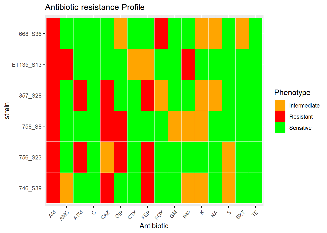
## TE S S S S S SVisualize
t<-data

t$ATB <- row.names(t) # creating "ATB" column, necessary for the melt() to work

t_m <- reshape2::melt(t, id.vars = "ATB")              #Reshape package

colnames(t_m) <- c("ATB","Strain","value") # giving relevant names to the melted table

#df_tm$ATB <- factor(df_tm$ATB, levels = c("AM", "AMC", "FEP", "CTX", "FOX", "CAZ", "ATM", "ETP", "CIP", "NA.", "SXT", "C", "TE", "GM", "K", "S", "Col"))

levels(factor(t_m$value)) # this helps to assign the colours
## [1] "I" "R" "S"ggplot2::ggplot(t_m, aes(ATB, Strain)) + geom_tile(aes(fill = factor(value), colour = c("white","white","white") ), colour = "white") + theme(legend.title=element_text(colour = "black", size = 12), axis.text.x = element_text(angle = 45, hjust=1, size=8)) + labs(title="Antibiotic resistance Profile", size = 15) + labs(x="Antibiotic",y="strain") + labs(fill='Phenotype') + scale_fill_manual(values=c("orange","red", "green"), labels= c('Intermediate', 'Resistant', 'Sensitive'))